Display Tab
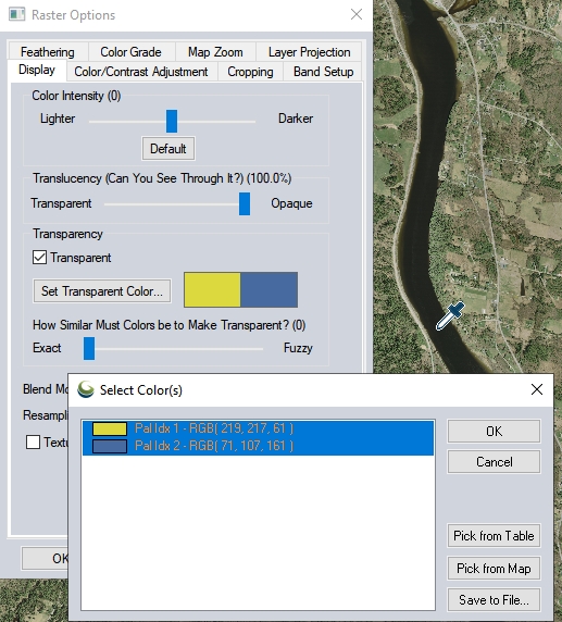
The Display tab (pictured below) specifies the color intensity (brightness/darkness), color transparency, blending, anti-aliasing, and texture mapping of the selected layers.
Access the display options from the control center using the  Layer Options toolbar button, or right clicking on the layer name and selecting Options. It will also open when double-clicking on the layer name. The Raster Options and Elevation options dialogs contain a display tab.

Color Intensity
The Color Intensity setting controls whether displayed pixels are lightened or darkened before being displayed. It may be useful to lighten or darken raster overlays in order to see overlaying vector data clearly.
Translucency
The Translucency setting controls to what degree the overlay displays the overlays underneath it. Settings closer to Transparent make the overlay increasingly more see-through, allowing you to blend overlapping data.
Transparency
In the Transparency section, the Transparent option allows a particular color (or colors) to be displayed transparently, making it possible to see through a layer to the layers underneath.
The Set Transparent Color... button allows the user to select the color to treat as transparent.
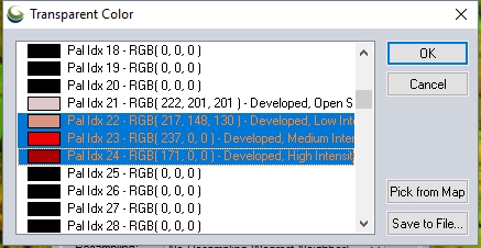
With palette files, the available colors will be automatically populated in the list on the left. Select multiple transparent colors using the CTRL or SHIFT key and clicking the palette colors. CTRL can also be used with the Pick from Map tool to pick multiple colors in a palette file.
With other raster files, the Transparent color list will be empty to begin with. Use the Pick from Map or Pick From Table buttons to add colors to the list. Highlighted colors will be set at transparent. Use the SHIFT or CTRL keys to highlight multiple transparent colors once picked.
Pick from Table - This option is available for imagery or elevation layers that do not contain a palette. This will display the Color selection dialog. Select a basic color, or use the settings on the right to fine tune the color by Hue, Saturation and Luminosity, or Red Green and Blue values.
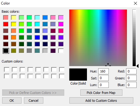
Add to Custom Colors – This adds the color to the list of custom colors, shown below the basic colors.
Pick Color From Map – when this option is selected the cursor will change to an eyedropper. Click on any 2D map to select the color value at the cursor location.
Save to File – This will save the list of colors to a palette file.
Load from File - Use this option to load color from an external file such as a pallet (.pal) file.
The Exact to Fuzzy slider in the Transparency section controls how similar to the selected transparent color(s) that a color in the image has to be before it is also treated as transparent. The Exact side means that only exact matches on color will be treated as transparent, moving the slider towards the Fuzzy side makes progressively less similar colors be treated as transparent. This is useful for getting rid of colors in lossy formats like JPG and ECW where the colors are not exact.
For Example: When viewing a DRG on top of a DOQ, making the white in the DRG transparent makes it possible to see much of the DOQ underneath.
To remove listed transparent colors, click Set Transparent Color and select a color from the list, then click the Delete key. To delete multiple colors at once, hold the ALT key and select multiple listed colors, then click the Delete key. To delete all colors, hold the SHIFT key and select the top most listed color and then select the bottom listed color, then click the Delete key.
Online Layer Detail Offset
The Online Layer Detail Offset allows for online layers to draw data at a lower resolution for faster display. The detail control of online layers will enable pulling data from lower or higher resolution layers, rather than the default screen resolution calculation.
Blend Mode
The Blend Mode setting controls
how an overlay is blended with underlying overlays, in addition to the
Translucency setting. These settings allow Photoshop-style filters to
be applied to overlays. The results from a particular blend mode with
different sets of overlays can often be difficult to predict. It is best
to experiment with different settings. The Hard
Light setting works well with satellite imagery overlaid on DEMs,
but the others can be quite useful as well.
Blend Mode Tip: The Apply Color setting is useful for applying color to a grayscale overlay, such
as using a low-resolution color LANDSAT image to colorize a high-resolution grayscale satellite image. The SPOT Natural Color blend mode combines the color channels in the topmost layer using the common algorithm for generating natural color imagery from images from the SPOT HRV multi-spectral sensor [Red = B2; Green = ( 3 * B1 + B3 ) / 4; Blue = ( 3 * B1 - B3 ) / 4]. The Pseudo Natural Color blend mode combines the color channels within a single image using a common algorithm for generating natural color imagery from CIR imagery. The Color to Grayscale blend mode converts a color image to grayscale.
Resampling
The Resampling option allows you to control how the color value for each displayed/export location is determined based on the values in the file.
To instead create a new layer with the applied filter, use the Apply Convolution Filter to Layer tool from the Analysis dropdown menu.
Filters /Resampling methods
When the pixels change size due to changes in resolution or reprojection, the filtering method determines how new pixel values are calculated. Some of these filters are good for highlighting edges, where "edges" are sudden changes in the intensity of pixels in an area of the image.
The following filtering methods are supported:
Nearest Neighbor - simply uses the value of the sample/pixel that a sample location is in. When resampling an image this can result in a stair-step effect, but will maintain exactly the original color values of the source image.
Box Average - the box average method simply find the average values of the nearest 4 (for 2x2), 9 (for 3x3), 16 (for 4x4), 25 (for 5x5), 49 (for 7x7), 64 (for 8x8), or 81 (for 9x9) ) pixels and use that as the value of the sample location. These methods are very good for resampling data at lower resolutions. The lower the resolution of your export is as compared to the original, the larger "box" size you should use.
Box Maximum - the box maximum methods simply find the maximum value of the nearest 4 (for 2x2), 9 (for 3x3), 16 (for 4x4), 25 (for 5x5), 49 (for 7x7), 64 (for 8x8), or 81 (for 9x9) pixels and use that as the value of the sample location. These methods are very good for resampling elevation data at lower resolutions so that the new terrain surface has the maximum elevation value rather than the average (good for terrain avoidance). The lower the resolution of the export file is as compared to the original, the larger "box" size that should be used.
Box Minimum - the box minimum methods simply find the minimum value of the nearest 4 (for 2x2), 9 (for 3x3), 16 (for 4x4), 25 (for 5x5), 49 (for 7x7), 64 (for 8x8), or 81 (for 9x9) pixels and use that as the value of the sample location. These methods are very good for resampling elevation data at lower resolutions so that the new terrain surface has the minimum elevation value rather than the average. The lower the resolution of the export file is as compared to the original, the larger "box" size that should be used.
Filter/Noise/Median - the Filter/Noise/Median methods simply find the median values of the nearest 4 (for 2x2), 9 (for 3x3), 16 (for 4x4), 25 (for 5x5), 49 (for 7x7), 64 (for 8x8), or 81 (for 9x9) pixels and use that as the value of the sample location. This resampling function is useful for noisy rasters, so outlier pixels do not contribute to the kernel value. Some common sources of raster noise are previous compression artifacts or irregularities of a scanned map/image.
Gaussian Blur - the Gaussian blur methods calculate the value to be displayed for each pixel based on the nearest 9 (for 3x3), 25 (for 5x5), or 49 (for 7x7) pixels. The calculated value uses the Gaussian formula that weights the values based on the distance to the reference pixel.
Box Mode (Most Common) - the Box Mode method sets the sample value to the most common value within the box , like the mode of the list of values. If there are multiple values with the same count, then if one matches the center value, that is kept. Otherwise just the first of the most common is used.
Smooth - the smoothing filter is used to smooth an image by reducing the contrast between neighboring pixels. It produces smooth images and the edges and corners are less accentuated. It is a weighted average where values closer to the center of the box are more heavily weighted. (Contrast this to Box Average where all values in the Kernel are weighted equally)
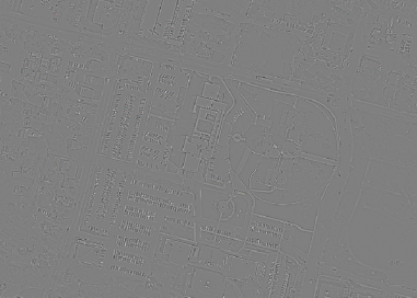
Sharpen - Sharpen filters (3x3 only) accentuate differences in a value with its neighbors, sharpening edges between objects. Examples and details on the sharpen filter variations are shown below.
-
Sharpen II (3x3) is similar to Sharpen (3x3), but the filter is more aggressive than Sharpen (3x3).
-
Sharpen High Pass (3x3, 5x5) - often used for edge enhancement. It accentuates the differences in pixel values compared to their neighboring pixels by calculating a weighted sum for each pixel in the image using a kernel neighborhood. It brings out the edges and boundaries between different features, making the image appear sharper. The kernel used in the filter (3x3, 5x5) determines size of the neighboring pixels (9, 25) that are included in the neighborhood and how much weight is given to each of them.
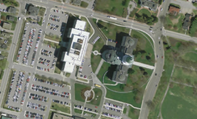
Sharpen Filter Examples
Sharpen Kernel Example Original 
Sharpen
0 -0.25 0 -0.25 2 -0.25 0 -0.25 0 
Sharpen II
-0.25 -0.25 -0.25 -0.25 3 -0.25 -0.25 -0.25 -0.25 
Sharpen (High Pass)
-1 -1 -1 -1 9 -1 -1 -1 -1 
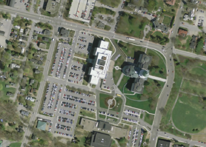
Gradient - the Gradient Filters (3x3 only) is used to detect edges in an image by calculating the gradient in a specified cardinal direction. Options include North, East, South, Northeast, and Northwest. When used on elevation data the generated layer will display with the gradient shader applied.
Gradient Kernel Example Terrain Example Image Original 
North
-1 -2 -1 0 0 0 1 2 1 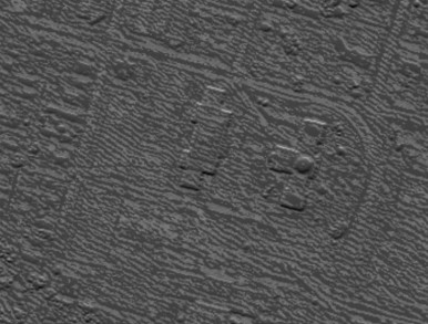
South
1 2 1 0 0 0 -1 -2 -1 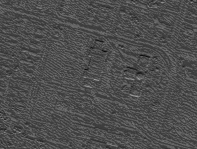
East
1
0 -1 2 0 -2 1 0 -1 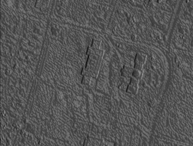
West
-1 0 1 -2 0 2 -1 0 1 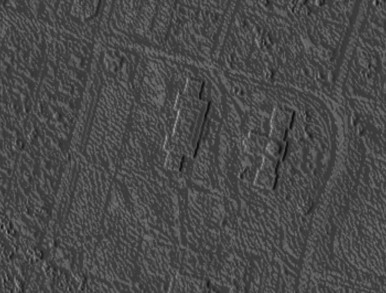
Northeast
0 -1 -2 1 0 -1 2 1 0 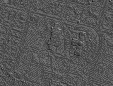
Northwest
-2 -1 0 -1 0 1 0 1 2 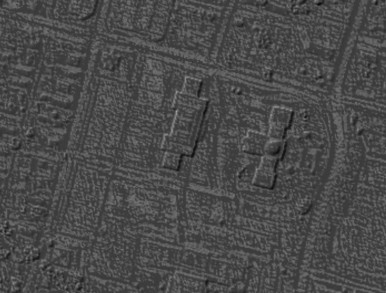
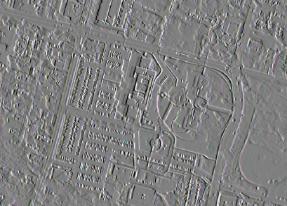
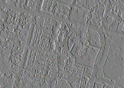
Laplacian (Edge Detection) - the Laplacian filter (3x3 or 5x5 only) is a second-order derivative operator, used to calculate the rate of change in the intensity of an image, and emphasizes areas of rapid intensity change, such as edges. It is a more sensitive edge detection method, often best applied to an image that has first been smoothed. When used on elevation data the generated layer will display with the gradient shader applied.
Laplacian Kernel Example Terrain Example Image Original 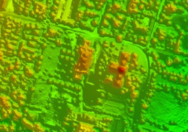

3x3
0 -1 0 -1 4 -1 0 -1 0 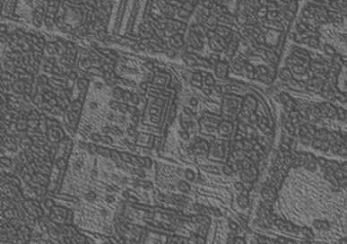
5x5
0 0 -1 0 0 0 -1 -2 -1 0 -1 -2 17 -2 -1 0 -1 -2 -1 0 0 0 -1 0 0 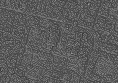
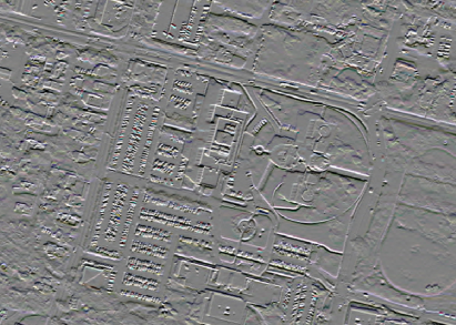
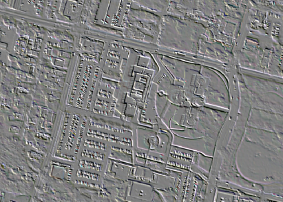
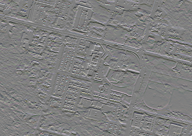
Line Detection- the Line Detection filters (3x3 only) can be used for edge detection similar to the Gradient Filters. These filters accentuate lines oriented in the specified direction ( either horizontal, vertical, or diagonal) while suppressing the others. When used on elevation data the generated layer will display with the gradient shader applied.
Line Detection Kernel Example Terrain Example Image Original 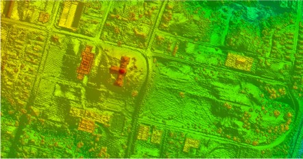
Horizontal
-1 -1 -1 2 2 2 -1 -1 -1 
Vertical
-1 0 -1 -1 2 -1 -1 2 -1 
Left Diagonal
2 -1 -1 -1 2 -1 -1 -1 2 
Right Diagonal
-1 -1 2 -1 2 -1 2 -1 -1 
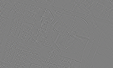
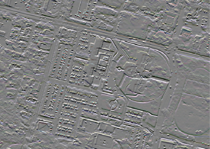
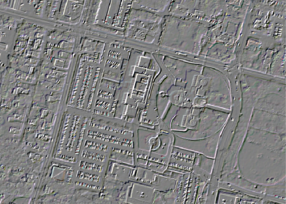
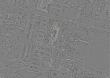
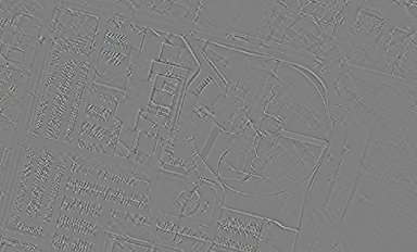
Sobel - Sobel filters are used for edge detection that involves a convolution of 3x3 kernel, for detecting either horizontal or vertical edges by multiplying the corresponding pixel values of the image with the kernel and summing them up. It results in an image where the intensity values of pixels are proportional to the strength of the directional edges in the original image. Edges are visible as extreme high/low values in the generated layer. When used on elevation data the generated layer will display with the gradient shader applied.
Sobel Kernel Example Terrain Example Image Original 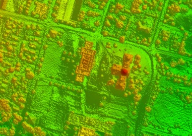

Horizontal
-1 -2 -1 0 0 0 1 2 1 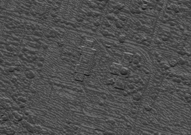
Vertical
-1 0 1 -2 0 2 -1 0 1 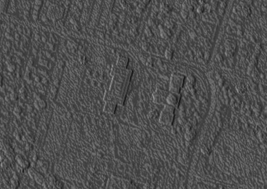
Bounds
Texture Map
The Texture
Map option allows a 2D raster overlay to be draped over loaded
3D elevation overlays. Selecting the check box causes the overlay to use
any available data from underlying elevation layers to determine how to
color the DRG or DOQ. The result is a shaded relief map.